Pi Play: Tracking Home Broadband Speed

I’ve been messing about with our Raspberry Pi 2 here in recent weeks. My first project was an SSH honeypot, built around the open-source honeypot kippo. I’ll post something on it in the next week or so. It was … entertaining.

The second, ongoing project is tracking and analyzing home broadband speed. I pay for Time Warner Ultimate Max XL Something Or Another, which is supposed to be 30 mbps down, and 5 mbps up. About 70% of the time that seems to be the case when I check, but at least 30% of the time it feel like it tests lower.

I generally use Ookla to test speeds, but that’s only when I remember, so I have no good data. Is it as bad as I think? Or am I just testing at bad times? Or am I only remembering the poor speeds? I really have no sense how bandwidth trends over the course of the day here – Time-Warner sure doesn’t provide it.

Enter my Raspberry Pi. I had long ago written a script to track home bandwidth, but it was a hack that ran on my router. (Trust me: Don’t do that.) This time I decided to host the scripts on the Pi, and store the data there too. I’m a Python guy, (insofar as I have any programming skills whatsoever, which I don’t) so that part was easy.

After some futzing about, I came up with this simple approach. I would use the speedtest-cli open source tool to grab hourly broadband data. I would store that in a text file. I would then use Python to take the data from the file and store it in sqlite.

The script for grabbing the data & running the tests isn’t mine. I just called the speedtest script (installed as above) from a cron process on the Pi. Here is the line from cron:

0 */1 * * * /usr/bin/python /usr/local/lib/python2.7/dist-packages/speedtest_cli.py --simple > /home/paul/speed.txt

In cron lingo, I’m calling the script every hour on the hour, and I’m using the “simple” flag for speedtest-cli . That mean it only returns three things: ping time, download speed, and upload speed. The data is then “piped” to the file “speed.txt” in my home folder. Its contents are overwritten every hour, & they look like this:

Ping: 24.903 ms
Download: 31.74 Mbit/s
Upload: 5.39 Mbit/s

I then created a second Python script to scrape that data file with a regular expression. It extracts the numbers, stores them in a database, and then updates a graph. I’ll give a brief overview of each of those steps in turn. Note first that this second script runs five minutes after the above one.

Here is the cron entry:

5 */1 * * * /usr/bin/python /home/paul/st.py >>/home/paul/st.log 2>&1

1) Extract the data. It’s a simple regular expression. I didn’t even bother to put in a loop – it just wasn’t worth it. I had to import the relevant Python packages first:

import re
import sqlite3 as lite
import sys
import time
import sqlite3 as lite
import plotly.plotly as py
import plotly
from plotly.graph_objs import *
import pandas as pd

And now extract the data:

lines = open('/home/paul/speed.txt').read().splitlines()
p = re.match("Ping: (.*?) ms", lines[0])
d = re.match("Download: (.*?) Mbit/s", lines[1])
u = re.match("Upload: (.*?) Mbit/s", lines[2])

2) Store the data in a database. I used sqlite because the data was so simple, and there was no need for concurrent users, etc. I won’t bore you with creating the data tables, etc. In addition to the three data fields, I have an auto-incrementing “id” field, plus a “sqltime” field that automatically stores the time (in GMT) of the latest update.

con = lite.connect('/home/paul/tw-speed.db')

with con:
    cur = con.cursor()  
    cur.execute('''INSERT INTO data(ping,download,upload) VALUES(?,?,?)''',(p.group(1),d.group(1),u.group(1)))

3) Update the graph. You could stop at the preceding step. After all, you’ve got the data, and you’re updating it with more data hourly. But it’s not much fun being unable to see the trends, so … a graph is required, at least for me. I’m a big fan of Plotly, a hosted graphing service, so I used it to host my graph.

First, extract the data back out of the sqlite database and put it in a Pandas dataframe:

with con:
    cur = con.cursor()
    cur.execute('SELECT id,ping,download,upload,datetime(sqltime, "localtime") FROM data')
    rows = cur.fetchall()
df = pd.DataFrame( [[ij for ij in i] for i in rows] )
df.rename(columns={0: 'id', 1: 'Ping', 2: 'Download', 3: 'Upload', 4:'Date'}, inplace=True);
df = df.sort(['Date'], ascending=[1]);

Next, set up the look and structure of the chart. This is all Plotly syntax, and it’s well-documented on the Plotly site:

trace1 = Scatter(
     x=df['Date'],
     y=df['Download'],
     name='Download',
)
trace2 = Scatter(
    x=df['Date'],
    y=df['Upload'],
    name='Upload',
    yaxis='y2'
)
layout = Layout(
    title="Time Warner Broadband Speed",
    xaxis=XAxis( title='Date' ),
    yaxis=YAxis(
        title='Download speed (mb/s)',
        range=[0,35]
    ),
    yaxis2=YAxis(
        title='Upload speed (mb/s)',
        range=[0,6],
        titlefont=Font(
            color='rgb(148, 103, 189)'
        ),
        tickfont=Font(
            color='rgb(148, 103, 189)'
        ),
        overlaying='y',
        side='right'
    )
)

Finally, update the graph with the latest data. Make sure you enter your Plotly username and key. There is one issue here though. Unless you make your graph public, only you will be able to see the graph you create, if you embed it somewhere other than Plotly’s site. (I have mine set private, and so it can only be seen on our internal network.)

py.sign_in('username', 'key')
data = Data([trace1,trace2])
fig = Figure(data=data, layout=layout)
py.plot(fig, filename='broadband speeds',world_readable=False)

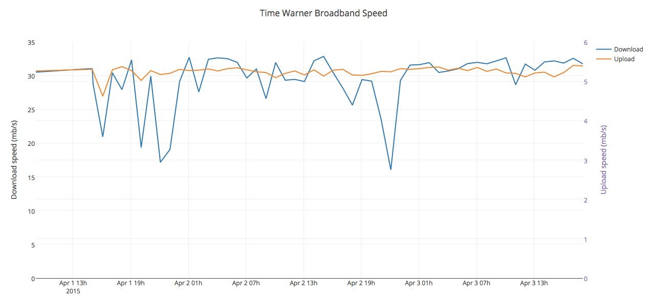
And that’s about it. Here is my graph, and it gets updated hourly by the scripts. You can see interesting trends, like how bandwidth declines every evening as my neighbors go mad with Netflix and other streaming services. You can also see, more importantly, that my recent bandwidth, while varying, has been acceptable. Curse you Time-Warner for providing what you said you would – but I won’t stop watching you.

Have fun. Enjoy tracking your bandwidth.